电力消耗预测
项目背景
企业用电需求预测一直是电力市场营销活动业务难点,大数据与云计算、人工智能等新技术相结合,给传统行业转型升级带来了新的机遇和思考。本项目主要用到开放扬中市高新区1000多家企业的历史用电量数据,通过模型算法预测该地区下一个月的每日总用电量。
数据采集
本项目主要用到开放扬中市高新区1000多家企业的历史用电量数据,直接在官网下载csv文件即可。
数据处理
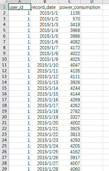
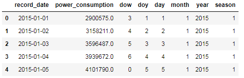
从上面的图可以看到,原始数据主要由3个维度组成:user_id,record_date,power_consumption,分别对应企业ID,日期以及用电量
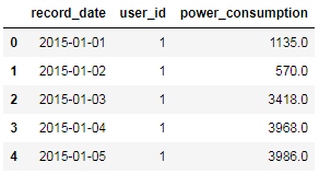
日期格式转换
因为原数据的日期是strting类型,所以我们需要把它格式转换
1 | import pandas as pd |
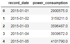
统计每日均值
1 | base_df = df[['record_date','power_consumption']].groupby(by='record_date').agg('sum') |
特征工程
因为数据只有3个维度,可能会造成欠拟合的情况,所以我们利用日期构建一些特征。
增加日期特征
1 | base_df['dow'] = base_df['record_date'].apply(lambda x: x.dayofweek) |
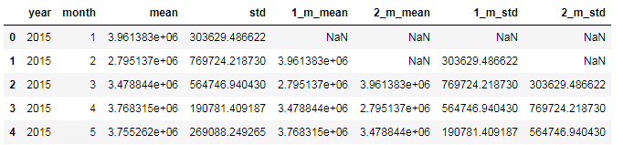
增加月度特征
1 | base_df_stats = new_df = base_df[['power_consumption','year','month']].groupby(by=['year', 'month']).agg(['mean', 'std']) |
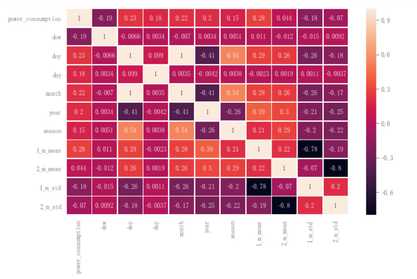
相关性检测
1 | import matplotlib.pyplot as plt |
数据分析
企业与用电量的关系
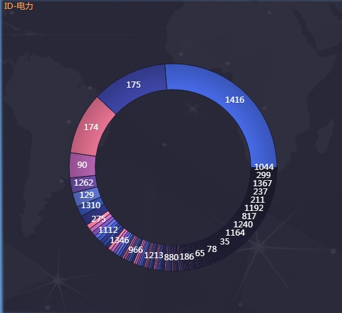
可以看到ID为1416,174,175的企业用电量很大
如果有必要可以把这3个企业单独分为1类做处理。
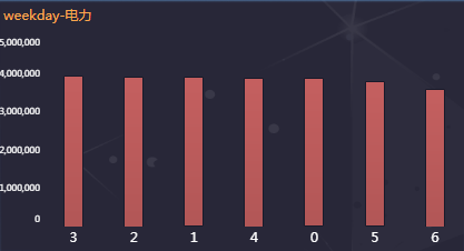
时间维度与用电量的关系


数据建模
在这个项目中,我们主要用到XGboost这个算法模型
训练模型
首先我们用模型默认的参数进行预测1
2
3
4
5
6
7
8
9
10
11
12
13
14
15df_finall = pd.read_excel('data_all.xlsx',sheet_name='V2')#加载数据
from sklearn.cross_validation import KFold, train_test_split
from xgboost import XGBRegressor
from sklearn import metrics
from sklearn.cross_validation import KFold, train_test_split
X = df_finall.iloc[:,1:-1]
X[['dow','doy','day','month','year','season']] = X[['dow','doy','day','month','year','season']]\
.astype(str)
y = df_finall.iloc[:,-1]
X_train, X_test, y_train, y_test = train_test_split(X.values, y.values, test_size=0.3)
xgb1 = XGBRegressor()
xgb1.fit(X_train,y_train)
test_predictions = xgb1.predict(X_test)
r2 = metrics.r2_score(y_test, test_predictions)
r2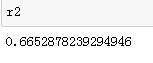
参数微调
因为XGBoost自带的参数较多,所以我们采用网格搜索的方式对参数进行微调。
- Step 1: 选择一组初始参数
1
xgb1 = XGBRegressor(eta=0.01, num_boost_round=50, colsample_bytree=0.5, subsample=0.5,objective='reg:linear',seed=27)
- Step 2: 改变
max_depth和min_child_weight.1
2
3
4
5xgb_param_grid = {'max_depth': list(range(4,9)), 'min_child_weight': list((1,3,6))}
grid = GridSearchCV(XGBRegressor(eta=0.01, num_boost_round=50, colsample_bytree=0.5, subsample=0.5,objective='reg:linear',seed=27),
param_grid=xgb_param_grid, cv=5)
grid.fit(X_train, y_train)
grid.grid_scores_, grid.best_params_, grid.best_score_网格搜索发现的最佳结果:1
2
3
4
5
6
7
8
9
10
11
12
13
14
15
16
17([mean: 0.66566, std: 0.11042, params: {'max_depth': 4, 'min_child_weight': 1},
mean: 0.65945, std: 0.10346, params: {'max_depth': 4, 'min_child_weight': 3},
mean: 0.65507, std: 0.08334, params: {'max_depth': 4, 'min_child_weight': 6},
mean: 0.67838, std: 0.09230, params: {'max_depth': 5, 'min_child_weight': 1},
mean: 0.65974, std: 0.09295, params: {'max_depth': 5, 'min_child_weight': 3},
mean: 0.65113, std: 0.08137, params: {'max_depth': 5, 'min_child_weight': 6},
mean: 0.68250, std: 0.08758, params: {'max_depth': 6, 'min_child_weight': 1},
mean: 0.66546, std: 0.10096, params: {'max_depth': 6, 'min_child_weight': 3},
mean: 0.65293, std: 0.09142, params: {'max_depth': 6, 'min_child_weight': 6},
mean: 0.67734, std: 0.08246, params: {'max_depth': 7, 'min_child_weight': 1},
mean: 0.66691, std: 0.09677, params: {'max_depth': 7, 'min_child_weight': 3},
mean: 0.66142, std: 0.08414, params: {'max_depth': 7, 'min_child_weight': 6},
mean: 0.67381, std: 0.11030, params: {'max_depth': 8, 'min_child_weight': 1},
mean: 0.67931, std: 0.09550, params: {'max_depth': 8, 'min_child_weight': 3},
mean: 0.66090, std: 0.08821, params: {'max_depth': 8, 'min_child_weight': 6}],
{'max_depth': 6, 'min_child_weight': 1},
0.6825025931707269)
{‘max_depth’: 6, ‘min_child_weight’: 1} - Step 3: 调节
gamma降低模型过拟合风险.1
2
3
4
5xgb_param_grid = {'gamma':[ 0.01 * i for i in range(0,5)]}
grid = GridSearchCV(XGBRegressor(eta=0.01, num_boost_round=50, colsample_bytree=0.5, subsample=0.5,objective='reg:linear',seed=27,max_depth=7,min_child_weight=1),
param_grid=xgb_param_grid, cv=5)
grid.fit(X_train, y_train)
grid.grid_scores_, grid.best_params_, grid.best_score_网格搜索发现的最佳结果:1
2
3
4
5
6
7([mean: 0.67462, std: 0.09512, params: {'gamma': 0.0},
mean: 0.67462, std: 0.09512, params: {'gamma': 0.01},
mean: 0.67462, std: 0.09512, params: {'gamma': 0.02},
mean: 0.67462, std: 0.09512, params: {'gamma': 0.03},
mean: 0.67462, std: 0.09512, params: {'gamma': 0.04}],
{'gamma': 0.0},
0.6746192263207629)
{‘gamma’: 0.0} - Step 4: 调节
subsample和colsample_bytree改变数据采样策略.1
2
3
4
5
6
7xgb_param_grid = {'subsample':[ 0.1 * i for i in range(6,10)],
'colsample_bytree':[ 0.1 * i for i in range(6,10)]}
grid = GridSearchCV(XGBRegressor(eta=0.01, num_boost_round=50, colsample_bytree=0.5, subsample=0.5,objective='reg:linear',seed=27,max_depth=7,
min_child_weight=1,gamma=0),
param_grid=xgb_param_grid, cv=5)
grid.fit(X_train, y_train)
grid.grid_scores_, grid.best_params_, grid.best_score_网格搜索发现的最佳结果:1
2
3
4
5
6
7
8
9
10
11
12
13
14
15
16
17
18([mean: 0.67014, std: 0.13270, params: {'colsample_bytree': 0.6000000000000001, 'subsample': 0.6000000000000001},
mean: 0.67302, std: 0.10802, params: {'colsample_bytree': 0.6000000000000001, 'subsample': 0.7000000000000001},
mean: 0.66858, std: 0.11634, params: {'colsample_bytree': 0.6000000000000001, 'subsample': 0.8},
mean: 0.67034, std: 0.11901, params: {'colsample_bytree': 0.6000000000000001, 'subsample': 0.9},
mean: 0.66074, std: 0.12567, params: {'colsample_bytree': 0.7000000000000001, 'subsample': 0.6000000000000001},
mean: 0.67163, std: 0.11620, params: {'colsample_bytree': 0.7000000000000001, 'subsample': 0.7000000000000001},
mean: 0.67011, std: 0.11888, params: {'colsample_bytree': 0.7000000000000001, 'subsample': 0.8},
mean: 0.67345, std: 0.10611, params: {'colsample_bytree': 0.7000000000000001, 'subsample': 0.9},
mean: 0.67388, std: 0.11610, params: {'colsample_bytree': 0.8, 'subsample': 0.6000000000000001},
mean: 0.67462, std: 0.10752, params: {'colsample_bytree': 0.8, 'subsample': 0.7000000000000001},
mean: 0.68473, std: 0.10995, params: {'colsample_bytree': 0.8, 'subsample': 0.8},
mean: 0.69456, std: 0.08956, params: {'colsample_bytree': 0.8, 'subsample': 0.9},
mean: 0.66677, std: 0.11420, params: {'colsample_bytree': 0.9, 'subsample': 0.6000000000000001},
mean: 0.66556, std: 0.10918, params: {'colsample_bytree': 0.9, 'subsample': 0.7000000000000001},
mean: 0.67706, std: 0.11681, params: {'colsample_bytree': 0.9, 'subsample': 0.8},
mean: 0.67529, std: 0.11429, params: {'colsample_bytree': 0.9, 'subsample': 0.9}],
{'colsample_bytree': 0.8, 'subsample': 0.9},
0.6945571414092301)
{‘colsample_bytree’: 0.8, ‘subsample’: 0.9} - Step 5: 调节学习率
learning_rate.1
2
3
4
5xgb_param_grid = {'learning_rate':[0.6,0.5,0.4,0.3,0.2,0.1,0.01,0.001]}
grid = GridSearchCV(XGBRegressor( num_boost_round=50,objective='reg:linear',seed=27,max_depth=7,
min_child_weight=1,gamma=0,colsample_bytree=0.8,subsample=0.9),param_grid=xgb_param_grid, cv=5)
grid.fit(X_train, y_train)
grid.grid_scores_, grid.best_params_, grid.best_score_网格搜索发现的最佳结果:1
2
3
4
5
6
7
8
9
10([mean: 0.56345, std: 0.18185, params: {'learning_rate': 0.6},
mean: 0.60402, std: 0.16560, params: {'learning_rate': 0.5},
mean: 0.67215, std: 0.13258, params: {'learning_rate': 0.4},
mean: 0.63116, std: 0.13087, params: {'learning_rate': 0.3},
mean: 0.62305, std: 0.16146, params: {'learning_rate': 0.2},
mean: 0.69456, std: 0.08956, params: {'learning_rate': 0.1},
mean: -12.66985, std: 4.34214, params: {'learning_rate': 0.01},
mean: -77.40167, std: 26.16110, params: {'learning_rate': 0.001}],
{'learning_rate': 0.1},
0.6945571414092301)
{‘learning_rate’: 0.1} - step 6:调节
n_estimators的棵数1
2
3
4
5xgb_param_grid = {'n_estimators':[50,100,200,300,400,500]}
grid = GridSearchCV(XGBRegressor( learning_rate=0.1,objective='reg:linear',seed=27,max_depth=7,
min_child_weight=1,gamma=0,colsample_bytree=0.8,subsample=0.9),param_grid=xgb_param_grid, cv=5)
grid.fit(X_train, y_train)
grid.grid_scores_, grid.best_params_, grid.best_score_网格搜索发现的最佳结果:1
2
3
4
5
6
7
8([mean: 0.69015, std: 0.08067, params: {'n_estimators': 50},
mean: 0.69456, std: 0.08956, params: {'n_estimators': 100},
mean: 0.69296, std: 0.09306, params: {'n_estimators': 200},
mean: 0.69270, std: 0.09327, params: {'n_estimators': 300},
mean: 0.69269, std: 0.09334, params: {'n_estimators': 400},
mean: 0.69270, std: 0.09335, params: {'n_estimators': 500}],
{'n_estimators': 100},
0.6945571414092301)
{‘n_estimators’: 100}
模型最终的参数为:最终评分:1
2
3
4
5
6
7XGBRegressor( learning_rate=0.1,
objective='reg:linear',
seed=27,max_depth=7,
min_child_weight=1,
gamma=0,
colsample_bytree=0.8,
subsample=0.9)1
2
3
4
5
6xgb3 = XGBRegressor( learning_rate=0.1,objective='reg:linear',seed=27,max_depth=7,
min_child_weight=1,gamma=0,colsample_bytree=0.8,subsample=0.9)
xgb3.fit(X_train,y_train)
test_predictions = xgb3.predict(X_test)
r2 = metrics.r2_score(y_test, test_predictions)
r21
0.7133043132603486